Mathematica is a powerful general CAS which is capable of generating models for 3D printing. Mathematica is able to export manifolds as STL and OBJ 3D data sets which can be read by CAD and 3D printing software. It is recommended to use Mathematica version 12 or higher. RegionPlot has computational errors in previous versions of Mathematica which may cause Mathematica to crash.
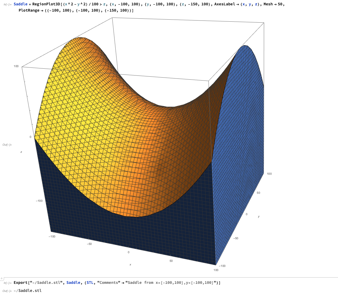
Saddle Example:
Export[“~/Saddle.stl”, Saddle, {STL, “Comments” -> “Saddle from x=[-100,100],y=[-100,100]”}]
In this example, a gridded surface is created for z=x2-y2. The surface is subdivided in both the X and Y axis with a mesh of 50 units.
The resulting saddle is then exported to the file “Saddle.stl” and includes a useful description in the data file.
The STL file can be edited in CAD software such as TinkerCad, or 3D printed directly via software such as Ultimaker Cura
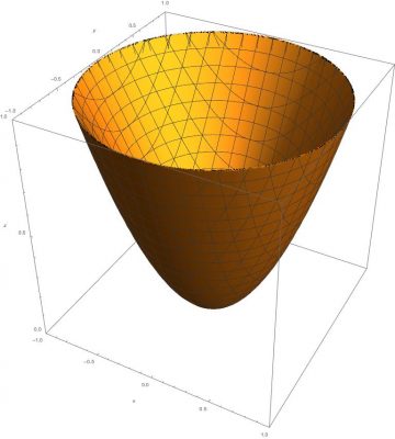
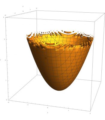
RegionPlot3D can also be used to perform boolean operations to plot the volume between between different functions; however, care must be used with parameters for the generation the resulting data sets. If parameters such as PlotPoints do not have sufficient values, the resulting geometry may be jagged, have topological errors, or have improperly curved boundaries as demonstrated by the example below for the region between a parabaloid and cone.
The example used the following equations for the region between the curves:
Parabaloid :=z >= (x^2 + y^2)
Cone := z <= =Sqrt[3x^2 +3y^2]
z >= (x^2 + y^2) &&
z <= Sqrt[3x^2 + 3y^2],
{x, -2, 2}, {y, -2, 2}, {z, 0, 4},
AxesLabel -> {x, y, z}, Mesh -> True,
PlotRange -> {{-2, 2}, {-2, 2}, {0, 4}}]
z >= (x^2 + y^2) &&
z <= Sqrt[3x^2 + 3y^2],
{x, -2, 2}, {y, -2, 2}, {z, 0, 4},
AxesLabel -> {x, y, z}, Mesh -> True,
PlotRange -> {{-2, 2}, {-2, 2}, {0, 4}},
PlotPoints->500]